Excel array formulas allow you to something that is counterintuitive to the rest of they way Excel works--perform an iterative calculation. In general, Excel allows you to create a formula that includes a reference to an array. In Excel, an array is a contiguous range of data either in the same row or the same column, like A1:E1 or B2:B124. Many functions in Excel have arguments that can only be a single cell. If you provide a range with multiple cells, it just looks at the upper-left corner of the range. For example,
=FIND(A1,B$1)
finds the string contained in cell A1 within the value shown in B$1. But if you do this
=FIND(A1:A10,B$1)
the function will only try to find the value of A1 within B$1. It will not attempt to look for all the values in the range A1:A10.
Other functions can accept a range of multiple cells, such as SUM and AVERAGE.
Microsoft has inexplicably never provided comprehensive documentation on this topic. Excel Help now points you to articles written by Excel luminaries John Walkenbach and Colin Wilcox, instead of their native help pages.
By the way, Excel has some formulas that will return an array if the argument is an array. One of these is TREND. TREND is used to analyze a series of data, usually with time as an independent variable, perform a least-squares regression, and then extrapolate the dependent variable for additional values.
SUMPRODUCT at its simplest sums the products (get it?) of each series of corresponding elements in its arguments, which are arrays. So suppose you have a list of 50 sales, with unit price in column A and number of units in column B. To calculate total sales, you could create formula in another column that multiplies the number in the same row in A times B, and then sum all of those formulas. Or you could use a single formula:
=SUMPRODUCT(A1:A50,B1:B50)
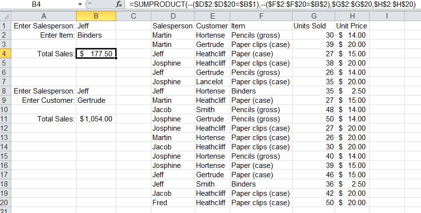
However, SUMPRODUCT can be very powerful when you go beyond this. For example, suppose you have a list of items sold. Each row has salesman, customer, item, units sold, and unit price. Say we want to let the user calculate the total value of a particualr product sold by a selected salesperson:
Cell B4 contains a SUMPRODUCT formula shown in the formula bar. It looks worse than it is. Let's break it down:
=$D$2:$D$20=$B$1
This part takes each element of the array $D$2:$D$20 and compares it to the value in $B$1. This comparison for equality returns TRUE or FALSE. But Excel won't do arithmetic on TRUE and FALSE values in a SUMPRODUCT formula. So we are going to force Excel to convert the result to a number. TRUE will be converted to 1, and FALSE will be converted to 0.
--($D$2:$D$20=$B$1)
How does this work? Putting a negative sign in front of the entire expression forces Excel to convert the logical value to a number to be able to apply an arithmetic operation to it (unary minus). But TRUE will then be converted to -1, so we add another negative sign to flip that over to be 1. Now the result is an array where the value is 1 every time the salesperson is Jeff.
We repeat the same thing to look for the item:
--($F$2:$F$20=$B$2)
So far we have two arrays that contain 0's and 1's. Remember that SUMPRODUCT calculates the sum of the product of these arrays. So if the salesman is Jeff and the product is Binders, the product is 1 x 1 = 1. Any other values will give 0.
We have two more values left: the quantity and unit price. When we multiply those, we get the total sale price, just as in our first example above. This total sales price is going to multiplied by a 1 if both salesman and item match, and a 0 otherwise. Therefore the sum of all those products is the total sales price of all Binders sold by Jeff.
There are some other functions that produce array results unexpectedly. As near as I can find this is an undocumented feature. Although it seems to have limited utility, I'll mention it here.
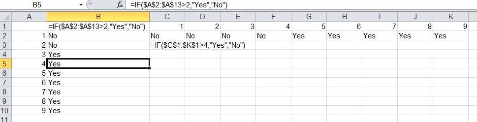
IF takes an expression for the If part, which it evaluates to be either TRUE or FALSE. If you use an array instead of a single cell in that expression, then IF will return an array. What does this mean? It means that if you use the same formula in continguous cells parallel to the referenced array, the formula will return the array element corresponding to the position where the formula is used. An example will make this much clearer. In Column A below there is a simple list of numbers. In column B, there is an IF function using an array in its If condition. The array is the list of numbers in column A. It tests to see if this array is greater than 2. Intuition would say, "IF isn't an array formula so it's only going to look at the top left cell, or A2." In fact, it will look at the cell in the same row as the IF formula. All of the cells in the range B2:B8 have exactly the same formula; that formula is shown in cell B1 and also in the formula bar (note that cell B5 is selected). The same thing works on an array in a row; you can see exactly the same phenomenon at work row-wise in the formulas in C2:K2.
I said this is of limited utility. That's because you can just as easily, and probably more clearly, use the following formula in B2:
=IF(A2>2,"Yes","No")
and then fill it down to B10 and get the same result. Using an array in that formula doesn't make it easier to understand (maybe even harder), and provides no other advantage that I can think of. But it's a behavior of Excel that is good to be aware of, especially if you are trying to debug someone else's worksheet.