Starting in Excel 2007, the user interface for managing Conditional Formatting changed dramatically. It took a little getting used to but it really does make more sense, and is much more powerful. It has some new little bells and whistles as far as the formatting itself, but the big improvement is being able to see all the rules and what cells they apply to.
However, Microsoft left out some details about how to write rules. The features that this article is about, which is the option I use the most, is "Use a formula to determine which cells to format." This allows you to write a custom formula that has the same syntax as a formula in an Excel cell. It must evaluate to TRUE or FALSE. If and only if it's TRUE, then the formatting rule that you specify will be applied. These formulas work almost the same as regular Excel formulas, but cell references mean something a little different.
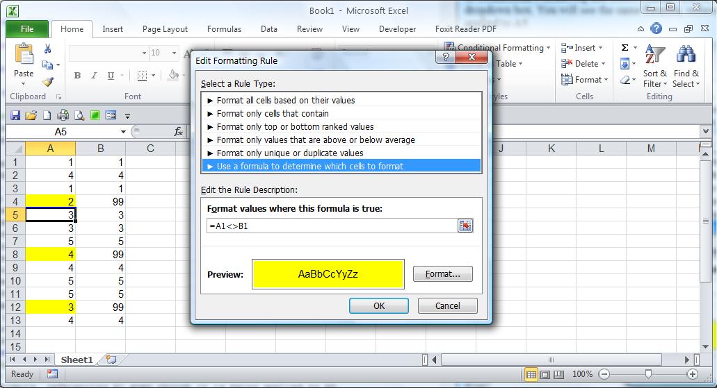
Suppose you have two columns of data in A and B, and you want to highlight any cells in column A where the value doesn't match the same row in B. You start by selecting the cells in column A, then add a conditional formatting rule. When you create a new rule, the default is that it applies to the selected cells (you can overwrite the default). You can use this formula:
=A1<>B1
Once you write this rule, now select any cell in column A—let's pick A5—then go back to Conditional Formatting and select Manage Rules, then Current Selection from the dropdown box. You will see the same formula, referencing A1, even though it is being applied to A5.
Why is this? When you select a range, then write a new Conditional Formatting rule for it, any reference to the upper left cell in the selected range will be interpreted to mean "any cell that this formula applies to." As the formula is applied to other cells, the other references will follow it along, the same way that Excel automatically adjusts references when you do a copy and paste. So when you are looking at cell A5, the formula that is really used to determine whether conditional formatting applies is
=A5<>B5
Note that not only is the row changed for the selected cell, but the row for B1 is B5, just as if you had copied a formula from A1 to A5. I am showing this formula only to illustrate how it works. You will never actually see this formula in Excel!
Let's expand the example to highlight cells in both columns. Now we need to define a formula that has A1 in the upper left, but will also make sense if we apply it to cells in column B. So we have to make those cell references use absolute column references:
=$A1<>$B1
Just as for Excel cell formulas, the $ means that it will use the same column reference whether it is testing a cell in column A or column B. It will always compare the value in column A to the value in column B regardless of which column has the value to be tested for formatting.
Let's take another simple example. Suppose you want to highlight any values in column A or column B that match a value in C1. You can write:
=A1=$C$1
Now we are using A1 as a relative reference, because we want it to mean "the cell I am testing to see if conditional formatting applies." Remember, it will be applied to every cell in column A and column B, even though it says A1. We have to use an absolute reference to C1so Excel doesn't try to relocate the reference as it evaluates different cells.
Once you understand these basic principles of writing conditional formatting formulas, you can extend it to more complex formulas. All the same functions available for Excel cells are available in conditional formatting functions, but you don't get the pop-up memory joggers that you get when writing a formula in a cell. So if you want to use a function that you're a little rusty on, look it up first. If your formula had invalid syntax, you will get an error when you try to save it but you won't get help to diagnose it.
A very effective trick is to develop the formula you want to use right in your worksheet. Pick a cell that's not being used and write the formula to refer to the cell in the upper left corner of the range you want to format. Once it has no errors, and says TRUE when you think the formatting should be applied, you can copy the formula from the formula bar (don't just copy the cell) and paste it into the conditional formatting formula bar. I'll use my simple example to show how this can be done. You can see that I've put the formula in column C and filled down. The result is TRUE in every row where I want the value in A to be highlighted. Then the formula can be copied from the top left corner of the range into the formula box for conditional formatting.
